An example showing how to do optimization with general constraints using SLSQP and cobyla.
Script output:
Optimization terminated successfully.    (Exit mode 0)
          Current function value: 2.47487373504
          Iterations: 5
          Function evaluations: 20
          Gradient evaluations: 5
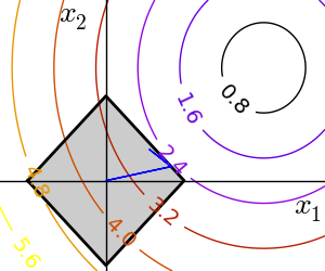
Python source code: plot_non_bounds_constraints.py
import numpy as np
import pylab as pl
from scipy import optimize

x, y = np.mgrid[-2.03:4.2:.04, -1.6:3.2:.04]
x = x.T
y = y.T

pl.figure(1, figsize=(3, 2.5))
pl.clf()
pl.axes([0, 0, 1, 1])

contours = pl.contour(np.sqrt((x - 3)**2 + (y - 2)**2),
                    extent=[-2.03, 4.2, -1.6, 3.2],
                    cmap=pl.cm.gnuplot)
pl.clabel(contours,
        inline=1,
        fmt='%1.1f',
        fontsize=14)
pl.plot([-1.5,    0,  1.5,    0, -1.5],
        [   0,  1.5,    0, -1.5,    0], 'k', linewidth=2)
pl.fill_between([ -1.5,    0,  1.5],
                [    0, -1.5,    0],
                [    0,  1.5,    0],
                color='.8')
pl.axvline(0, color='k')
pl.axhline(0, color='k')

pl.text(-.9, 2.8, '$x_2$', size=20)
pl.text(3.6, -.6, '$x_1$', size=20)
pl.axis('tight')
pl.axis('off')

# And now plot the optimization path
accumulator = list()

def f(x):
    # Store the list of function calls
    accumulator.append(x)
    return np.sqrt((x[0] - 3)**2 + (x[1] - 2)**2)


def constraint(x):
    return np.atleast_1d(1.5 - np.sum(np.abs(x)))

optimize.fmin_slsqp(f, np.array([0, 0]),
                       ieqcons=[constraint, ])

accumulated = np.array(accumulator)
pl.plot(accumulated[:, 0], accumulated[:, 1])

pl.show()
Total running time of the example: 0.08 seconds ( 0 minutes 0.08 seconds)
